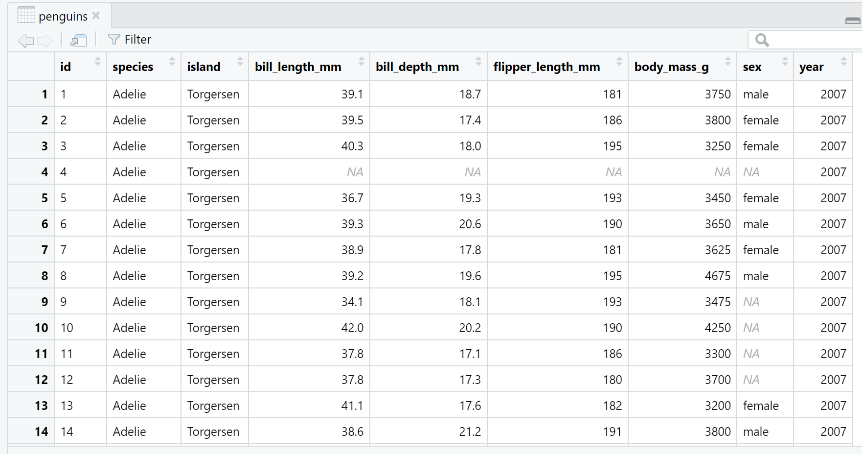
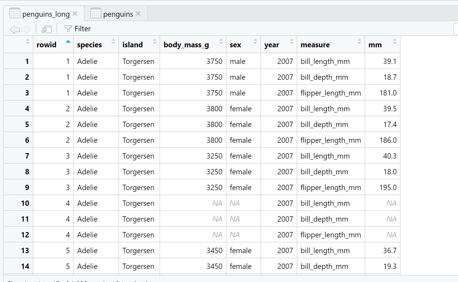
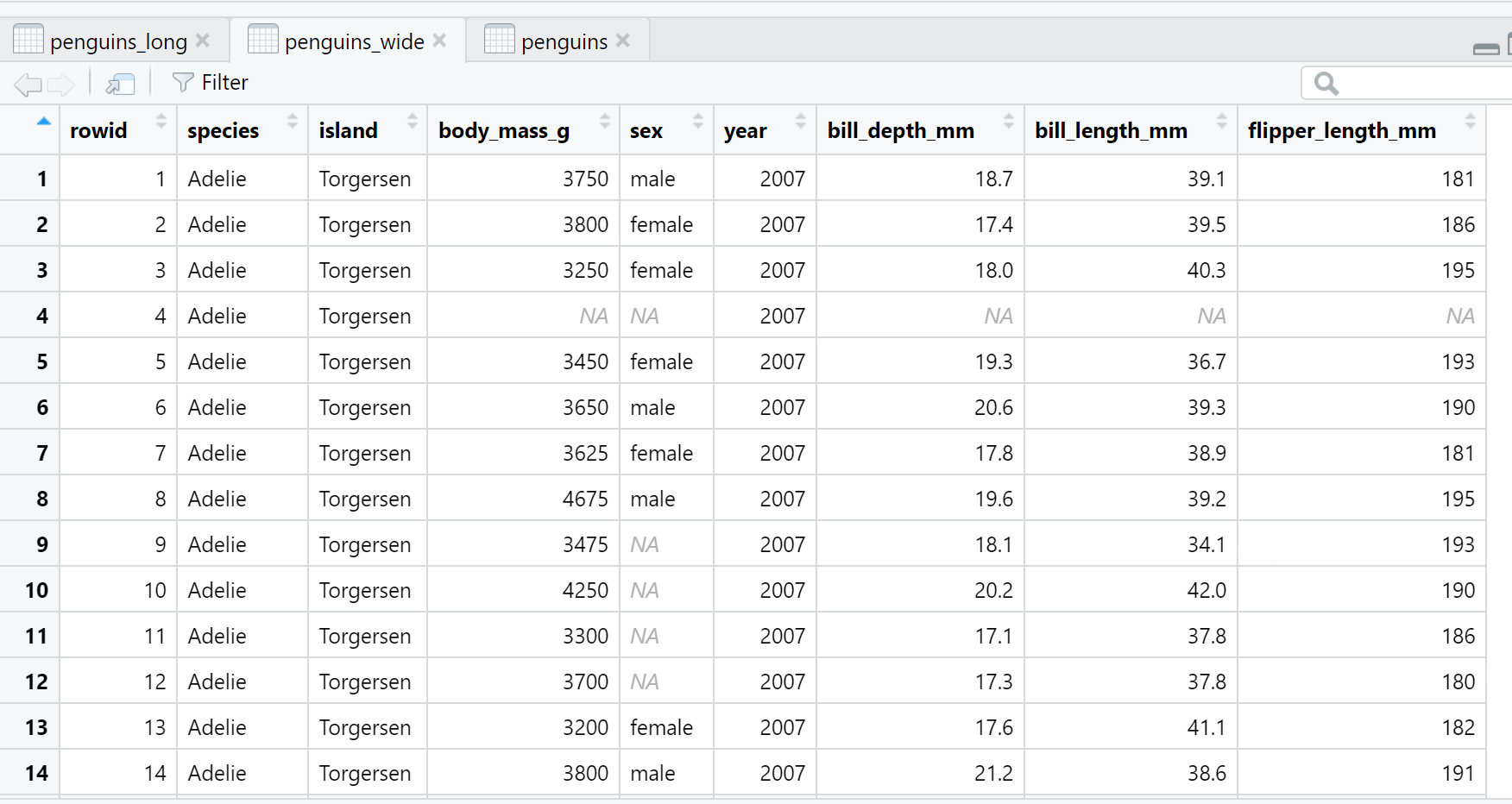
Import and Tidy

Session 2a

Author

Affiliation

Zixi Chen, PhD

NYU-Shanghai

1 Workflow in Tidyverse R

What is tidyverse? Do you recall the package section we’ve learnt in the last class? tidyverse is a meta package that loads nine core packages and other that share a design philosophy, common grammar, and data structure. It will make your R-learning as a beginner more intuitive and effective.

Tip

Read more: Why Tidyverse (for beginners.)

1.1 Tidyverse workflow

Figure 1 shows what a typical data science process using Tidyverse would look like.

Fig. 1: A typical model of data science process using Tidyverse retrieved from https://www.tidyverse.org

Commonly, a typical Tidyverse workflow involves six components and each component is facilitated by corresponding core Tidyverse packages. You first import or load your data into R from a file or web application programming interface (API) and then wrangle the raw data by tidying and transforming it. Along the way, you visualize and model the wrangled data to further explore and understand your data. With a deep understanding of your data descriptively, visually, and analytically, you can communicate your results to others.

This workflow is supported by Tidyverse’s nine core packages (eight original ones and lubridate) and many others. In this R session 2, we will explore the whole workflow with a few relevant Tidyverse packages.

library(tidyverse)

Warning: package 'tidyverse' was built under R version 4.3.3

Warning: package 'ggplot2' was built under R version 4.3.3

Warning: package 'tidyr' was built under R version 4.3.3

Warning: package 'dplyr' was built under R version 4.3.3

── Attaching core tidyverse packages ──────────────────────── tidyverse 2.0.0 ──
✔ dplyr     1.1.4     ✔ readr     2.1.5
✔ forcats   1.0.0     ✔ stringr   1.5.1
✔ ggplot2   3.5.1     ✔ tibble    3.2.1
✔ lubridate 1.9.3     ✔ tidyr     1.3.1
✔ purrr     1.0.2     
── Conflicts ────────────────────────────────────────── tidyverse_conflicts() ──
✖ dplyr::filter() masks stats::filter()
✖ dplyr::lag()    masks stats::lag()
ℹ Use the conflicted package (<http://conflicted.r-lib.org/>) to force all conflicts to become errors

Understanding warning messages

When working with R, you’ll encounter two types of important feedback messages: warning and error messages.

Warning messages are like yellow traffic lights, which alert you to potential issues but don’t stop code execution. As you’re loading tidyverse, you see a warning message appear since there are conflicts between functions: “dplyr::filter() masking stats::filter()”.

Error messages are like red traffic lights, which completely stop code execution and indicate something is fundamentally wrong. They are usually shown with an “Error:” prefix. We need to resolve these errors before code can proceed. GenAI is helpful for debugging errors. We will see a few examples in our later learning.

1.2 Structure of R Session 2

Using the tidyverse framework and grammar, we kick off the flowchart with import and tidy (as a part of wrangling) in Week 3. We will then continue the data wrangling and focus on the transform in Week 4.

In Week 5, we will introduce a tidyverse package called rvest to scrap the web data. We will present visualization basics using ggplot2 in Week 6.

2 Data import using readr

Empirical data analysis starts with importing data. In here, we use a Twitter data set, “tweets_dave” provided in Text Mining with R as an example. You can access the data page by clicking here and then click the “Raw” button on the right upper box, which will direct you to a new page. We will use this page’s URL later.

To start with, we can use read_delim function to read the most common types of csv or tsv files. We also can read files directly from a complete URL. Working with more specifically noted files, we can use read_csv() to read the comma-delimited csv files, read_csv2() to read the semicolon-separated csv files, and read_tsv to read the tab-separated tsv files.

Before importing the data, let’s take a quick look at the arguments of read_delim from here.

#first try
drob_tweets<-read_delim(file="https://raw.githubusercontent.com/dgrtwo/tidy-text-mining/master/data/tweets_dave.csv")

Rows: 4174 Columns: 10
── Column specification ────────────────────────────────────────────────────────
Delimiter: ","
chr (5): timestamp, source, text, retweeted_status_timestamp, expanded_urls
dbl (5): tweet_id, in_reply_to_status_id, in_reply_to_user_id, retweeted_sta...

ℹ Use `spec()` to retrieve the full column specification for this data.
ℹ Specify the column types or set `show_col_types = FALSE` to quiet this message.

Let’s then check how the variables were specified.

spec(drob_tweets)

cols(
  tweet_id = col_double(),
  in_reply_to_status_id = col_double(),
  in_reply_to_user_id = col_double(),
  timestamp = col_character(),
  source = col_character(),
  text = col_character(),
  retweeted_status_id = col_double(),
  retweeted_status_user_id = col_double(),
  retweeted_status_timestamp = col_character(),
  expanded_urls = col_character()
)

The identification variables, such as `tweet_id=col_double()`, were imported as numerical variables, which might lose information, such as the leading 0 or being converted to scientific notions. I suggest importing the id variables as character variables. So let’s re-import the data by specifying the types of id variables.

#getting the arguments specified
drob_tweets<-read_delim(file="https://raw.githubusercontent.com/dgrtwo/tidy-text-mining/master/data/tweets_dave.csv", 
                        col_types = cols(tweet_id =col_character(),
                                         in_reply_to_status_id = col_character(),
                                         in_reply_to_user_id = col_character(),
                                         timestamp = col_datetime(format = "%Y-%m-%d %H:%M:%S %z"),
  source = col_character(),
  text = col_character(),
  retweeted_status_id = col_character(),
  retweeted_status_user_id = col_character(),
  retweeted_status_timestamp = col_datetime("%Y-%m-%d %H:%M:%S %z"),
  expanded_urls = col_character()))
drob_tweets

# A tibble: 4,174 × 10
   tweet_id in_reply_to_status_id in_reply_to_user_id timestamp           source
   <chr>    <chr>                 <chr>               <dttm>              <chr> 
 1 8161085… <NA>                  <NA>                2017-01-03 02:26:59 "<a h…
 2 8158926… <NA>                  <NA>                2017-01-02 12:08:59 "<a h…
 3 8156415… <NA>                  <NA>                2017-01-01 19:31:17 "<a h…
 4 8156247… <NA>                  <NA>                2017-01-01 18:24:36 "<a h…
 5 8153681… <NA>                  <NA>                2017-01-01 01:24:50 "<a h…
 6 8153369… 815320862660366336    3230388598          2016-12-31 23:20:43 "<a h…
 7 8149858… <NA>                  <NA>                2016-12-31 00:05:45 "<a h…
 8 8148868… 814881114233794560    14254939            2016-12-30 17:32:30 "<a h…
 9 8145464… 814545877016580096    24228154            2016-12-29 18:59:32 "<a h…
10 8145454… 814545134012407808    24228154            2016-12-29 18:55:47 "<a h…
# ℹ 4,164 more rows
# ℹ 5 more variables: text <chr>, retweeted_status_id <chr>,
#   retweeted_status_user_id <chr>, retweeted_status_timestamp <dttm>,
#   expanded_urls <chr>

Working with Date-Time variables in R

It is best to specify any date-time type of variables when importing the data. This will help you retrieve time-related information much more efficiently later.

The above example showed how to specify the col_datetime(). Call ?col_datetime() to see how readr parses date and time variables.

The other two packages from Tidyverse, lubridate and clock, provide a variety of functions for working with date and time.

Fig.2 Artwork retrieved from allisonhorst.com

2.1 Take a glimpse of the data

Check whether we have the raw data read in as a data frame.

is_tibble(drob_tweets) 

[1] TRUE

Let’s then take a glimpse of this data by knowing its rows (i.e., observations) and columns (i.e., variables).

glimpse(drob_tweets)

Rows: 4,174
Columns: 10
$ tweet_id                   <chr> "816108564720812032", "815892641820901376",…
$ in_reply_to_status_id      <chr> NA, NA, NA, NA, NA, "815320862660366336", N…
$ in_reply_to_user_id        <chr> NA, NA, NA, NA, NA, "3230388598", NA, "1425…
$ timestamp                  <dttm> 2017-01-03 02:26:59, 2017-01-02 12:08:59, …
$ source                     <chr> "<a href=\"http://twitter.com/download/ipho…
$ text                       <chr> "RT @ParkerMolloy: 2017 is off to quite a s…
$ retweeted_status_id        <chr> "816082588137881600", "776081137722650628",…
$ retweeted_status_user_id   <chr> "634734888", "2842614819", "69133574", "756…
$ retweeted_status_timestamp <dttm> 2017-01-03 00:43:45, 2016-09-14 15:32:16, …
$ expanded_urls              <chr> "https://twitter.com/ParkerMolloy/status/81…

View(drob_tweets)

Activity 1

How many rows and columns are in this data? What do these variables mean?

2.1.1 Codebook

What do these variables mean? Let’s look at the Tweet Data Dictionary documented on the X developer platform. You may also read similar codebooks in other designed data sets (e.g., social surveys). The codebooks, or data dictionaries, are critical to building effective and reproducible data analysis projects. It is always better to create a codebook detailing the meaning of your column’s variables at the very early stage of building a project and update it along the way.

2.1.2 Missing objects

You might notice that many NAs pop out in the data, representing missing values. So, an NA in the in_reply_to_status_id variable means that this row of tweets is not a reply.

2.2 Importing other formats data

Data sources can be stored in various formats, such as Excel or txt files. As we’ve gone through read_delim(), you can explore what other functions like read_csv() can be used for importing different data formats. In addition to the readr package, many other packages are available for reading specific data formats, depending on your data conditions. GenAI might be a good resource for finding alternative packages and functions to help you import data if readr does not work.

3 Tidying data

Raw big data is rarely ready to use. They are normally created for other reasons rather than research. Most often, we tidy and transform data simultaneously. The package tidyr serves to facilitate the process of creating tidy data.

require(tidyr) # check if the library tidyr is loaded.
#Since tidyr is from tidyverse,we should have it loaded. 

Fig. 3 Artwork retrieved from allisonhorst.com

“Tidying your data means storing it in a consistent form that matches the semantics of the dataset with how it is stored. In brief, when your data is tidy, each column is a variable and each row is an observation.

Tidy data is important because the consistent structure lets you focus your efforts on answering questions about the data, not fighting to get the data into the right form for different functions.

–https://r4ds.hadley.nz/intro

Do you remember the palmerpenguins data we used last week? In the following, we demonstrate some useful functions to tidy this data set. Later, we will switch back to the drob_tweets data to show data transformation.

library(palmerpenguins) 
data("penguins")

# force(penguins)

Let’s add a unique identifier to each penguin before we move on.

penguins <- rowid_to_column(penguins) # this function comes from the tibble package. 

glimpse(penguins)

Rows: 344
Columns: 9
$ rowid             <int> 1, 2, 3, 4, 5, 6, 7, 8, 9, 10, 11, 12, 13, 14, 15, 1…
$ species           <fct> Adelie, Adelie, Adelie, Adelie, Adelie, Adelie, Adel…
$ island            <fct> Torgersen, Torgersen, Torgersen, Torgersen, Torgerse…
$ bill_length_mm    <dbl> 39.1, 39.5, 40.3, NA, 36.7, 39.3, 38.9, 39.2, 34.1, …
$ bill_depth_mm     <dbl> 18.7, 17.4, 18.0, NA, 19.3, 20.6, 17.8, 19.6, 18.1, …
$ flipper_length_mm <int> 181, 186, 195, NA, 193, 190, 181, 195, 193, 190, 186…
$ body_mass_g       <int> 3750, 3800, 3250, NA, 3450, 3650, 3625, 4675, 3475, …
$ sex               <fct> male, female, female, NA, female, male, female, male…
$ year              <int> 2007, 2007, 2007, 2007, 2007, 2007, 2007, 2007, 2007…

View the data at the top-left panel.

View(penguins)  

Fig.4 Penguins data structure

3.1 Reshape

3.1.1 From wide format to long format

As you can tell from the data structure, each row represents the observation values of a penguin. These observations include three common attributes of bill length and depth and flipper length. Now, we want to reform this data such that these three attributes are combined together as a single variable. We use pivot_longer() to do this task.

penguins_long<-tidyr::pivot_longer(penguins,
                            cols = bill_length_mm:flipper_length_mm,# names of columns to transform
               names_to = "measure", # new column name for the original column names
               values_to = "mm", # new column name for the values
               values_drop_na = FALSE) # not removing the missing observations

View(penguins_long)

Fig.4 Reshaping the penguins data set from wide format to long format

3.1.2 From long format to wide format

The function pivot_wider() is a complement to pivot_longer().

penguins_wide <-pivot_wider(penguins_long, 
                            names_from = "measure",  # column containing the new column names
              values_from = "mm", # column containing the values
              values_fill = NA ) # fill missing values with NA

Penguins_wide should look the same as the original Penguins data set.

View(penguins_wide)

Fig.5 Reshaping penguins long data to wide format

Note

pivot_longer() and pivot_wider() were introduced in tidyr 1.0.0 as more intuitive replacements for the older reshape functions of gather() and spread().

While gather() and spread() still works, it’s recommended to use pivot_*() functions as they provide clearer syntax and additional functionality for reshaping data.

3.2 Uniting and separating columns

Creating a new variable, “description,” that gathers the information of species and island.

penguins_unite<-unite(penguins, 
                 col="description", # the name of the new column
                c(species, island), # you can also use spcies:island
               # remove=F,
                 sep = ", ")

head(penguins_unite)

# A tibble: 6 × 8
  rowid description   bill_length_mm bill_depth_mm flipper_length_mm body_mass_g
  <int> <chr>                  <dbl>         <dbl>             <int>       <int>
1     1 Adelie, Torg…           39.1          18.7               181        3750
2     2 Adelie, Torg…           39.5          17.4               186        3800
3     3 Adelie, Torg…           40.3          18                 195        3250
4     4 Adelie, Torg…           NA            NA                  NA          NA
5     5 Adelie, Torg…           36.7          19.3               193        3450
6     6 Adelie, Torg…           39.3          20.6               190        3650
# ℹ 2 more variables: sex <fct>, year <int>

Activity 2

Can you unite the variables sex and year into one new variable?

Let’s separate the description variable using separate_wider_delim().

penguins_sep_wide<-separate_wider_delim(penguins_unite, 
                                        cols = description, 
                                        delim = ", ", 
                                        names=c("species", "island"))

It should be the same as the original format.

head(penguins_sep_wide)

# A tibble: 6 × 9
  rowid species island    bill_length_mm bill_depth_mm flipper_length_mm
  <int> <chr>   <chr>              <dbl>         <dbl>             <int>
1     1 Adelie  Torgersen           39.1          18.7               181
2     2 Adelie  Torgersen           39.5          17.4               186
3     3 Adelie  Torgersen           40.3          18                 195
4     4 Adelie  Torgersen           NA            NA                  NA
5     5 Adelie  Torgersen           36.7          19.3               193
6     6 Adelie  Torgersen           39.3          20.6               190
# ℹ 3 more variables: body_mass_g <int>, sex <fct>, year <int>

As you may have noticed in the separation function’s name, we can separate the description variable into the long format. Do you remember the previous penguins_long data structure? These two functions did the same thing here.

penguins_sep_long<-separate_longer_delim(penguins_unite, 
                                        cols = description, 
                                        delim = "," 
                                        )

In this way, each penguin has two rows of descriptions, one for species and the other one for island. We won’t use this data structure for understanding penguins. However, this function is useful when you data has a concatenated categorical variable, such as a variable indicating a series of years “2019,2020,2021”. Then you probably want to separate it and reshape the data into a long format for any longitudinal analysis.

View(penguins_sep_long)

Fig.7 Separating description to long format